Spatial Inequality in Road Casualty Risk under london Vision Zero Framework

1. Research Context

Transport for London’s Vision Zero strategy sets an ambitious target of eliminating all deaths and serious injuries on the city’s transport network by 2041 (TfL, 2018). Rooted in the Swedish Vision Zero philosophy — which holds that loss of life on the road is ethically unacceptable and preventable through systemic design rather than individual behaviour change (Tingvall and Haworth, 1999) — the programme places responsibility squarely on infrastructure designers and policymakers rather than on road users themselves. Achieving its targets requires more than reducing aggregate casualty numbers: it demands an understanding of where risk concentrates and why.

The spatial distribution of road casualties is well established as non-random. Research across multiple urban contexts has demonstrated that road injury risk varies systematically with urban form, land use, traffic exposure, and socio-economic context (Graham and Glaister, 2003; Morency et al., 2012). In dense, mixed-use environments — characteristic of inner London — the intersection of high pedestrian and cyclist volumes with complex road networks tends to produce elevated and spatially concentrated casualty risk (Noland and Quddus, 2004). These patterns are not simply a function of population size: even after controlling for exposure, spatial structure plays a significant independent role (Quddus, 2008). Spatial analysis is therefore essential for identifying high-risk areas, targeting interventions, and allocating resources efficiently — a point increasingly recognised in urban road safety policy (WHO, 2017).

This project investigates two related questions:

• RQ1: Are road casualty incidence patterns spatially clustered across London MSOAs, and where are the main high-risk areas located?
• RQ2: Do local clustering patterns indicate persistent spatial inequality in road casualty risk that warrants targeted Vision Zero interventions?

The analysis draws on TfL road casualty data (2024), 2021 MSOA boundaries, and Census 2021 socio-demographic variables. Middle Super Output Areas (MSOAs) are used as the primary spatial unit, balancing resolution with statistical stability and allowing consistent integration of Census-derived covariates.

2. Analytical Approach

The analysis proceeds in three stages, each building on the previous.

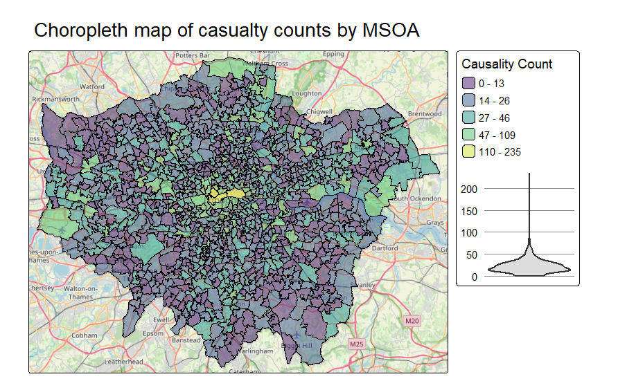
Exploratory Spatial Data Analysis (ESDA) establishes whether the spatial distribution of casualties departs from randomness. Casualty counts are aggregated to MSOAs and examined through choropleth mapping and density surfaces, providing a descriptive baseline and motivating formal statistical testing — consistent with standard ESDA practice in urban health and safety research (Anselin, 1999).

Prior to modelling, the distribution of each explanatory variable was examined to assess skewness and inform any necessary transformations. The no-car rate exhibited strong right skew and was log-transformed to improve linearity and variance stability in the OLS model.

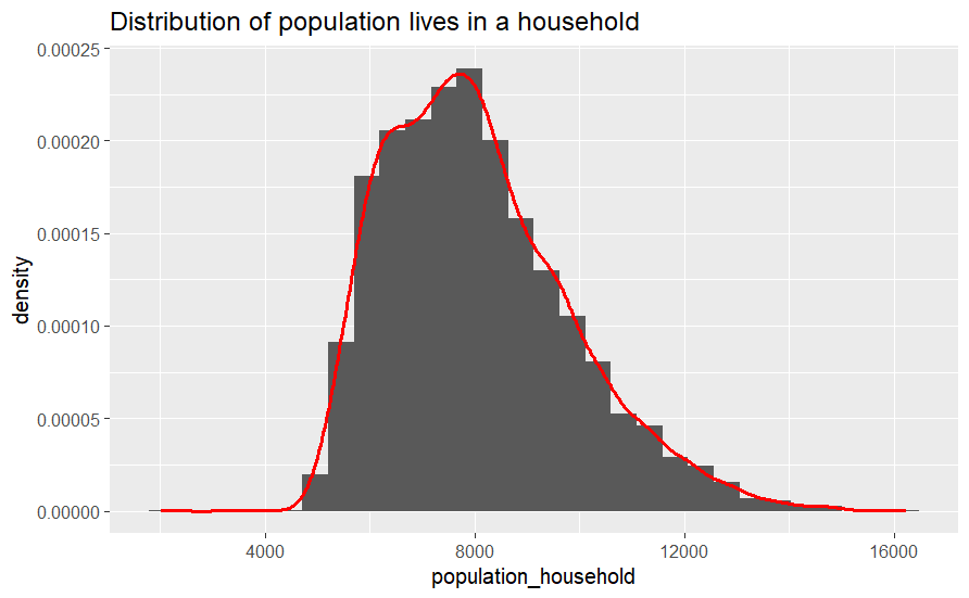
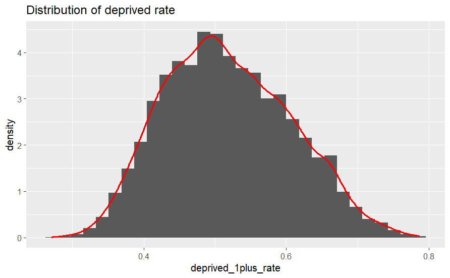
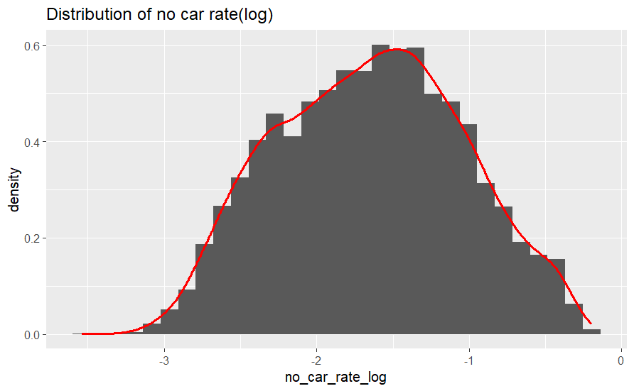
Spatial Autocorrelation quantifies the degree and structure of clustering. Global Moran’s I assesses whether high- and low-risk MSOAs are systematically co-located across the city (Moran, 1950; Cliff and Ord, 1981). Local Moran’s I (LISA) and Getis–Ord Gi* statistics then identify the specific locations of significant clusters and hotspots (Anselin, 1995; Getis and Ord, 1992). A contiguity-based Queen spatial weights matrix is used throughout, with row standardisation applied to ensure comparability across areas with different numbers of neighbours — a standard specification in area-based spatial analysis (Bivand, Pebesma and Gómez-Rubio, 2013).

Explanatory Modelling uses OLS regression to assess whether socio-demographic characteristics — household deprivation, car availability, and residential population — explain observed spatial variation in casualty rates. Variable selection follows prior research linking socio-economic context to road injury risk: deprivation is associated with greater exposure to road danger and lower access to safe infrastructure (Graham and Glaister, 2003), while car availability proxies travel behaviour and mode-specific exposure patterns (Mindell et al., 2012).

Residual diagnostics then test whether spatial dependence persists after controlling for these factors. Because OLS residuals show significant positive spatial autocorrelation (Moran’s I ≈ 0.32, p < 0.001), a Spatial Error Model (SEM) is adopted. SEM is appropriate here because spatial dependence arises from omitted contextual factors — road network complexity, land-use intensity, historical infrastructure decisions — that are spatially structured but not directly measured, rather than from direct spillover effects between neighbouring MSOAs (Anselin, 1988; LeSage and Pace, 2009). This distinction between spatial error and spatial lag dependence follows standard diagnostic practice in applied spatial econometrics (Anselin et al., 1996).

3. Key Findings

Global Moran’s I for casualty density is 0.55 (p < 0.001), confirming strong and statistically significant spatial clustering across London MSOAs: high-risk areas tend to be surrounded by other high-risk areas, and low-risk areas cluster similarly. This result is consistent with evidence from other major urban contexts showing persistent spatial concentration of road injury risk (Noland and Quddus, 2004; Quddus, 2008).

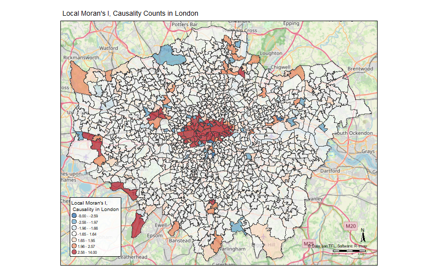
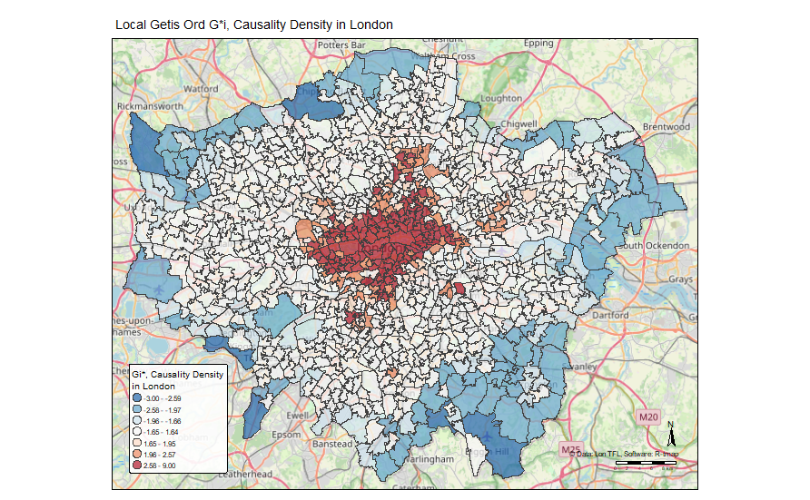
Local spatial statistics reveal that High–High clusters are concentrated in inner London, while Low–Low clusters dominate much of outer London. This inner–outer gradient reflects well-documented differences in road environment complexity, pedestrian and cyclist exposure, and traffic intensity between central and peripheral urban areas (Graham and Glaister, 2003; Loukaitou-Sideris, Liggett and Sung, 2007). The LISA and Gi* maps below illustrate both the location and intensity of these clusters.

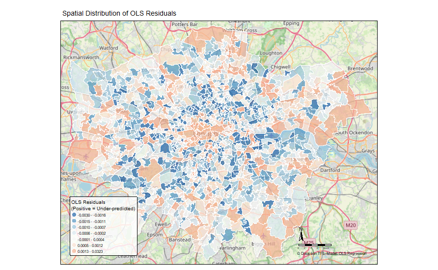
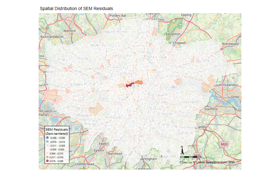
The SEM produces a spatial error parameter of λ = 0.57 (p < 0.001), confirming that strong spatially structured unobserved factors drive casualty risk beyond what socio-demographic variables alone can explain. SEM residuals show no significant spatial autocorrelation (Moran’s I ≈ 0.002, p = 0.44), validating the model specification (Anselin, 1988). The modest explanatory power of the OLS model (adjusted R² ≈ 0.11) is consistent with prior area-level road casualty research (Quddus, 2008), reflecting both the stochastic nature of traffic injuries and the absence of direct built-environment measures such as road network density and junction complexity. Crucially, residual diagnostics reveal that the OLS model fails to capture the underlying spatial structure of the data — a well-recognised limitation of standard regression when applied to spatially structured outcomes (LeSage and Pace, 2009). Comparing the OLS and SEM residual maps below makes this contrast explicit.

Among the explanatory variables, car availability shows a positive and significant association with casualty rates, consistent with evidence that lower car ownership correlates with greater reliance on walking, cycling, and public transport — modes with higher per-trip injury exposure in mixed urban environments (Mindell et al., 2012). Household deprivation shows a negative coefficient once spatial dependence is controlled for, suggesting that its influence operates indirectly through spatially clustered infrastructure and land-use factors, rather than as a direct and independent driver of risk (Morency et al., 2012).

4. Policy Implications

The persistence of High–High clusters in inner London — even after controlling for observed socio-demographic characteristics — points to a form of structural spatial inequality in road safety outcomes. Certain neighbourhoods are systematically more exposed to risk, reflecting cumulative pressures linked to mobility demand, urban density, and infrastructure design. This reinforces the Vision Zero principle that responsibility lies with system designers rather than road users (Tingvall and Haworth, 1999; WHO, 2017), and aligns with broader critiques of purely behavioural or enforcement-led safety strategies (Elvik, 2001).

These findings directly support targeted rather than uniform intervention. TfL’s Vision Zero Action Plan explicitly prioritises high-risk corridors and junctions (TfL, 2018), and the spatial clustering identified here provides empirical grounding for that place-based allocation. Research on urban road safety programmes suggests that geographically focused investment — in speed reduction, junction redesign, and protected infrastructure for pedestrians and cyclists — is both more cost-effective and more equitable than city-wide measures applied uniformly across heterogeneous risk environments (Elvik, 2001; Beyer and Ker, 2009).

5. Limitations

Several limitations should be noted. Casualty rates are normalised by residential population as a proxy for exposure, which may underestimate true risk in areas with high non-residential travel or visitor footfall. Road network variables — density, junction complexity, pedestrian infrastructure — were not incorporated into the regression models, and likely account for a portion of the variance absorbed by the spatial error term; future work should incorporate OpenStreetMap or Ordnance Survey network data to test this directly. The analysis is cross-sectional and exploratory, and observed associations should not be interpreted as causal effects. Extending the framework to a longitudinal design with fuller built-environment measurement would substantially improve causal identification (Quddus, 2008).

References

Anselin, L. (1988) Spatial Econometrics: Methods and Models. Dordrecht: Kluwer Academic Publishers.

Anselin, L. (1995) ‘Local indicators of spatial association — LISA’, Geographical Analysis, 27(2), pp. 93–115.

Anselin, L. (1999) ‘Interactive techniques and exploratory spatial data analysis’, in Longley, P.A. et al. (eds) Geographical Information Systems: Principles, Techniques, Management and Applications. New York: Wiley, pp. 251–264.

Anselin, L., Bera, A.K., Florax, R. and Yoon, M.J. (1996) ‘Simple diagnostic tests for spatial dependence’, Regional Science and Urban Economics, 26(1), pp. 77–104.

Beyer, F.R. and Ker, K. (2009) ‘Street lighting for preventing road traffic injuries’, Cochrane Database of Systematic Reviews, (1). doi: 10.1002/14651858.CD004728.pub2.

Bivand, R.S., Pebesma, E. and Gómez-Rubio, V. (2013) Applied Spatial Data Analysis with R. 2nd edn. New York: Springer.

Cliff, A.D. and Ord, J.K. (1981) Spatial Processes: Models and Applications. London: Pion.

Elvik, R. (2001) ‘Area-wide urban traffic calming schemes: A meta-analysis of safety effects’, Accident Analysis & Prevention, 33(3), pp. 327–336.

Getis, A. and Ord, J.K. (1992) ‘The analysis of spatial association by use of distance statistics’, Geographical Analysis, 24(3), pp. 189–206.

Graham, D.J. and Glaister, S. (2003) ‘Spatial variation in road pedestrian casualties: The role of urban scale, density and land-use mix’, Urban Studies, 40(8), pp. 1591–1607.

LeSage, J. and Pace, R.K. (2009) Introduction to Spatial Econometrics. Boca Raton: CRC Press.

Loukaitou-Sideris, A., Liggett, R. and Sung, H.-G. (2007) ‘Death on the crosswalk: A study of pedestrian–automobile collisions in Los Angeles’, Journal of Planning Education and Research, 26(3), pp. 338–351.

Mindell, J.S., Anciaes, P.R., Dhanani, A., Stockton, J., Jones, P., Haklay, M., Groce, N., Scholes, S., Vaughan, L. and Lam, K.B.H. (2012) ‘Using triangulation to assess a suite of tools to measure community severance’, Journal of Transport Geography, 60, pp. 119–129.

Moran, P.A.P. (1950) ‘Notes on continuous stochastic phenomena’, Biometrika, 37(1/2), pp. 17–23.

Morency, P., Gauvin, L., Plante, C., Fournier, M. and Morency, C. (2012) ‘Neighborhood social inequalities in road traffic injuries: The influence of traffic volume and road design’, American Journal of Public Health, 102(6), pp. 1112–1119.

Noland, R.B. and Quddus, M.A. (2004) ‘A spatially disaggregate analysis of road casualties in England’, Accident Analysis & Prevention, 36(6), pp. 973–984.

Quddus, M.A. (2008) ‘Modelling area-wide count outcomes with spatial correlation and heterogeneity: An analysis of London crash data’, Accident Analysis & Prevention, 40(4), pp. 1486–1497.

Tingvall, C. and Haworth, N. (1999) Vision Zero: An ethical approach to safety and mobility. Paper presented at the 6th ITE International Conference on Road Safety & Traffic Enforcement, Melbourne.

Transport for London (2018) Vision Zero for London. London: Transport for London. Available at: https://tfl.gov.uk/corporate/safety-and-security/road-safety/vision-zero (Accessed: 1 March 2024).

World Health Organization (2017) Save LIVES: A road safety technical package. Geneva: World Health Organization.